Dear all,
I am trying to set up a distribution for a binary RV \mathbf{x} \in \{ 0, 1\}^k:
P(\mathbf{x} \mid \boldsymbol p) = \prod^k_i Bernoulli(x_i \mid p_i)
for a mixture of images. The code of the distribution is below:
multivariate_bernoulli_distribution <- R6Class(
"multivariate_bernoulli_distribution",
inherit = distribution_node,
public = list(
initialize = function(prob, dim) {
prob <- as.greta_array(prob)
dim <- check_dims(prob, target_dim = dim)
super$initialize("multivariate_bernoulli", dim, discrete = TRUE)
self$add_parameter(prob, "prob")
},
tf_distrib = function(parameters, dag) {
prob <- parameters$prob
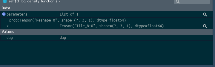
log_prob <- function(x) {
sum(x * log(prob) + (1 - x) * log(1 - prob))
}
list(log_prob = log_prob, cdf = NULL, log_cdf = NULL)
},
tf_cdf_function = NULL,
tf_log_cdf_function = NULL
)
)
When I test the distribution everything seems to work out, only the sampling throws an error:
n <- 25
p <- 3
prob <- beta(1, 1, p)
d <- matrix(rbinom(n * p, 1, .1), n)

for (i in seq(nrow(d)))
{
  distribution(d[i,]) <- multivariate_bernoulli(prob)
}

m <- model(prob)
plot(m)
samples <- mcmc(m)

 Error in py_call_impl(callable, dots$args, dots$keywords) :
  TypeError: Input 'y' of 'Sub' Op has type float64 that does not match type float32 of argument 'x'
Any idea how I could solve this?
Thanks,
Simon