Gaussian process in greta (Matern covariance)

As mentioned over on Github I am fiddling with spatial models a la: https://becarioprecario.bitbucket.io/spde-gitbook/ch-intro.html#sec:intro

Below is the code I could come up with inspired from: https://mc-stan.org/docs/2_19/stan-users-guide/fit-gp-section.html:

cMatern <- function(h, nu, kappa) {
  intt <- ifelse(h > 0, besselK(h * kappa, nu) * (h * kappa)^nu / 
           (base::gamma(nu) * 2^(nu - 1)), 1) 
  #intt <- intt * sigma
  return(intt)
}

# simulate some data
n <- 200
pts <- cbind(s1 = sample(1:n / n - 0.5 / n)^2,
             s2 = sample(1:n / n - 0.5 / n)^2)
dmat <- as.matrix(dist(pts))

# model parameter 
beta0 <- 10
sigma2e <- 0.3
sigma2u <- 5
kappa <- 7
nu <- 1

mcor <- cMatern(dmat, nu, kappa) 
mcov <- sigma2e * diag(nrow(mcor)) + mcor * sigma2u

R <- chol(mcov)
y1 <- beta0 + drop(crossprod(R, rnorm(n))) 

# greta modelling
## parameters
beta_0 <- normal(0, 1)
sigma_e <- cauchy(0, 5, truncation = c(0, Inf))
sigma_u <- cauchy(0, 5, truncation = c(0, Inf))
kappa <- normal(0, 1)
nu <- normal(0, 1)
eta <- normal(0, 1)

# linear predictor derivation
K <- cMatern(dmat, nu, kappa) 
K <- K * sigma_u
diag(K) <- diag(K) + 1e-9
L_K <- chol(K)
f <- L_K * eta + beta_0
# model
distribution(y1) <- normal(f, sigma_e)

Which does no work as I get the following error: “Error: cannot convert objects with missing or infinite values to greta_arrays”

Browsing through the greta forum this could be an interesting place to start.

Yup, you can definitely do GPs, that’s one of the main reasons I originally wrote greta! There’s a prototype extension package https://github.com/greta-dev/greta.gp to make these models easier, but it’s currently halfway through a refactor and doesn’t work with the current version of greta. Hoping to polish it off soon, because it’s a nice example of the sort of simple interface you can create with an extension package.

The reason your code isn’t working is that you are passing greta arrays into a bunch of functions for which there aren’t yet greta equivalents: ifelse, besselK, and base::gamma. Bessel K and gamma functions could easily be added to greta (once I work out what to call the gamma function without it being confused with the distribution), and I could probably get ifelse to work.

However, I never usually work with the full Matern covariance, because nu is really hard to estimate from data. This full version of the Matern covariance can’t be fitted in INLA either; nu has to specified. It should definitely be possible though, so let me know if you really want that and we can work out a covariance function for it.

For now, here’s a simpler example using a Matern 3/2 kernel (ie. nu fixed at 3/2).

Simulate data:

# Matern 3/2 correlation (no marginal variances added)
matern32 <- function (distances, lengthscale) {
  a <- sqrt(3 * distances ^ 2) / lengthscale
  (1 + a) * exp(-a)
}

# simulate some data
n <- 200
pts <- cbind(s1 = sample(1:n / n - 0.5 / n)^2,
             s2 = sample(1:n / n - 0.5 / n)^2)
dmat <- as.matrix(dist(pts))

# model parameter
beta0 <- 10
sigma2e <- 0.3
sigma2u <- 5
lengthscale <- 1/7

mcor <- matern32(dmat, lengthscale)
mcov <- sigma2e * diag(nrow(mcor)) + mcor * sigma2u

R <- chol(mcov)
y1 <- beta0 + drop(crossprod(R, rnorm(n)))

Fit Matern GP with the linear predictor approach as in your code. Note eta needs to be a length n vector, you need to matrix-multiply it with L_K, and R’s chol() (and therefore greta’s) actually returns the upper triangular matrix, so needs to be transposed to get the lower triangular matrix. I use the one_by_one argument to greta to deal with Cholesky decomposition failures with bad parameter sets.

library(greta)

beta_0 <- normal(0, 1)
sigma_e <- cauchy(0, 5, truncation = c(0, Inf))
sigma_u <- cauchy(0, 5, truncation = c(0, Inf))
lengthscale <- normal(0, 1, truncation = c(0, Inf))
eta <- normal(0, 1, dim = n)

# linear predictor
K <- matern32(dmat, lengthscale)
K <- K * sigma_u ^ 2
K <- K + diag(n) * 1e-9
L_K <- t(chol(K))
f <- L_K %*% eta + beta_0

distribution(y1) <- normal(f, sigma_e)

m <- model(beta_0, lengthscale, sigma_u)
draws <- mcmc(m, one_by_one = TRUE)

This parameterisation has a latent Gaussian process, and then the data are observed with additional error on top of that GP. Since the response is Gaussian in this case, it’s much nicer to reparameterise as having the data drawn from the Gaussian process but with extra marginal variance. Which is actually how you simulated the data. Note this won’t work with non-Gaussian observation models

The following does away with the eta parameter, doesn’t need jitter to be added to the kernel, and samples much more nicely:

beta_0 <- normal(0, 1)
sigma_e <- cauchy(0, 5, truncation = c(0, Inf))
sigma_u <- cauchy(0, 5, truncation = c(0, Inf))
lengthscale <- normal(0, 1, truncation = c(0, Inf))

# covariance matrix
K <- matern32(dmat, lengthscale)
K <- K * sigma_u ^ 2
K <- K + diag(n) * sigma_e ^ 2

# define a multivariate normal on the data *rowwise*, so that observations are
# correlated (each row is an independent MVN)
mu <- beta_0 + zeros(1, n)
ty <- t(y1)
distribution(ty) <- multivariate_normal(mu, K)

m <- model(beta_0, lengthscale, sigma_u)
draws <- mcmc(m, one_by_one = TRUE)

OK, I figured now was the time to get greta.gp working.

There’s a new branch and pull request open which depends on greta 0.3.1, which is itself still a release candidate (waiting on CRAN to accept) and pull request. You can install both by doing:

remotes::install_github("greta-dev/greta@rc_0_3_1")
remotes::install_github("goldingn/greta.gp@roll_forward")

Hopefully these will both be the master branches (and on CRAN, for greta) in a couple of days so those installation instructions will become redundant.

Here’s how you would do the same two models with greta.gp:

linear predictor (latent Gaussian process) version:

library(greta)
library(greta.gp)

beta_0 <- normal(0, 1)
sigma_e <- cauchy(0, 5, truncation = c(0, Inf))
sigma_u <- cauchy(0, 5, truncation = c(0, Inf))
lengthscale <- normal(0, 1, truncation = c(0, Inf))

K <- mat32(lengthscale, sigma_u ^ 2)
f_gp <- gp(pts, K, tol = 1e-9)
f <- f_gp + beta_0

distribution(y1) <- normal(f, sigma_e)

m1 <- model(beta_0, lengthscale, sigma_u)
draws1 <- mcmc(m1, one_by_one = TRUE)

observed Gaussian process version:

beta_0 <- normal(0, 1)
sigma_e <- cauchy(0, 5, truncation = c(0, Inf))
sigma_u <- cauchy(0, 5, truncation = c(0, Inf))
lengthscale <- normal(0, 1, truncation = c(0, Inf))

# covariance matrix
K1 <- mat32(lengthscale, sigma_u ^ 2)
K2 <- white(sigma_e ^ 2)
K <- K1 + K2

# define a multivariate normal on the data *rowwise*, so that observations are
# correlated (each row is an independent MVN)
mu <- beta_0 + zeros(1, n)
sigma <- K(pts)
ty <- t(y1)
distribution(ty) <- multivariate_normal(mu, sigma)

m2 <- model(beta_0, lengthscale, sigma_u)
draws2 <- mcmc(m2, one_by_one = TRUE)

A nice thing about this is that you can use greta.gp::project() to get a greta array for GP values in new locations, and greta::calculate() to get posterior samples for them. So you can easily do Gaussian process prediction to new locations even if you didn’t know the prediction locations before sampling.

s_seq <- seq(0, 1, length.out = 10)
pts_new <- expand.grid(s1 = s_seq,
                       s2 = s_seq)
f_gp_mn_new <- project(f_gp, pts_new)
f_mn_new <- f_gp_mn_new + beta_0
f_mn_new_draws <- calculate(f_mn_new, draws1)
f_mn_new_est <- colMeans(as.matrix(f_mn_new_draws))

That only works with the first one of these examples though. You have to do prediction yourself for the latter case (observed GP with noise):

K_xstar_x <- K1(pts_new, pts)
K_xstar_xstar <- K1(pts_new, pts_new)
i_sigma <- solve(sigma)
f_mn_new <- beta_0 + K_xstar_x %*% (i_sigma %*% as.matrix(y1))

f_mn_new_draws <- calculate(f_mn_new, draws2)
f_mn_new_est <- colMeans(as.matrix(f_mn_new_draws))

Note that both of these only compute posterior estimates of the mean of the GP at these locations, not realisations of the functions drawn from the GP. You’d need to calculate the posterior covariance matrix and draw more samples from a multivariate normal again to get posterior realisations of the function values.

1 Like

Oops, moving too fast! Accepted on CRAN now, so you can do:

remotes::install_github("greta-dev/greta")
remotes::install_github("goldingn/greta.gp")

Wow thanks a lot for the super fast response and happy to hear that this is integrated in an already developed package. I’ll have a try.

Should the second line rather be:

remotes::install_github("greta-dev/greta.gp")

Yes it should, thanks!

Ok, I tried this a bit and the code works fine, yet I get quite some bad mcmc sampling for the model parameters. I tried increasing the warmup and sample number to 4000 but the chains still look less than optimal (divergent iterations).

Do you have some tips on how to improve the sampling for such model?

what was the code that produced this?

I just retook the code you wrote earlier:

# matern32 correlation function
matern32 <- function (distances, lengthscale) {
  a <- sqrt(3 * distances ^ 2) / lengthscale
  (1 + a) * exp(-a)
}

# simulate some data
n <- 200
pts <- cbind(s1 = sample(1:n / n - 0.5 / n)^2,
             s2 = sample(1:n / n - 0.5 / n)^2)
dmat <- as.matrix(dist(pts))

# model parameter
beta0 <- 10
sigma2e <- 0.3
sigma2u <- 5
lengthscale <- 1/7

mcor <- matern32(dmat, lengthscale)
mcov <- sigma2e * diag(nrow(mcor)) + mcor * sigma2u

R <- chol(mcov)
y1 <- beta0 + drop(crossprod(R, rnorm(n)))

# greta modelling
library(greta)
library(greta.gp)

beta_0 <- normal(0, 5)
sigma_e <- cauchy(0, 5, truncation = c(0, Inf))
sigma_u <- cauchy(0, 5, truncation = c(0, Inf))
lengthscale <- normal(0, 10, truncation = c(0, Inf))

K <- mat32(lengthscale, sigma_u ^ 2)
f_gp <- gp(pts, K, tol = 1e-9)
f <- f_gp + beta_0

distribution(y1) <- normal(f, sigma_e)

m1 <- model(beta_0, lengthscale, sigma_u)
draws1 <- mcmc(m1, one_by_one = TRUE, warmup = 4000, n_sample = 4000)```

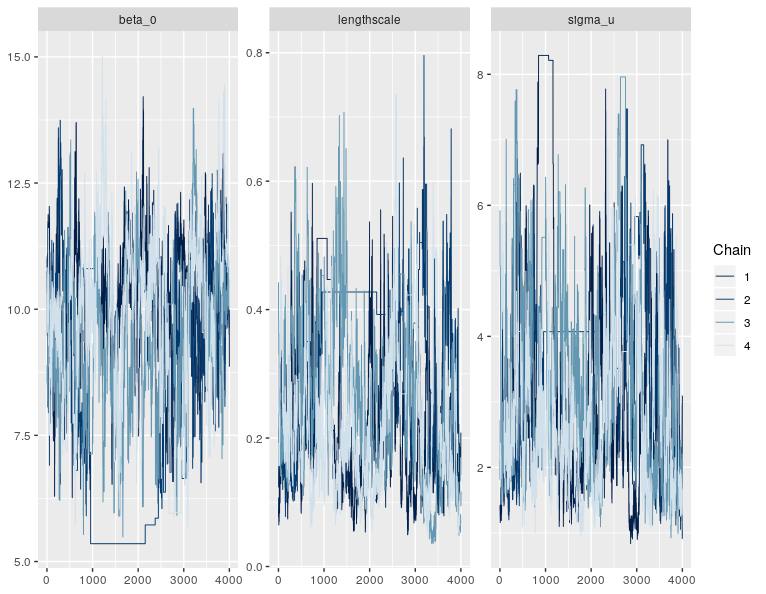
Right, it looks like the posterior for this model has an awkward geometry, so the sampler is getting a bit stuck in some points. This isn’t very surprising for GP models - there’s often some non-identifiability in the parameters, e.g. between the lengthscale and variance components. Or between the GP and the intercept.

Two options here, the most general one first, then a GP-specific one second:

Option 1. tune the sampler

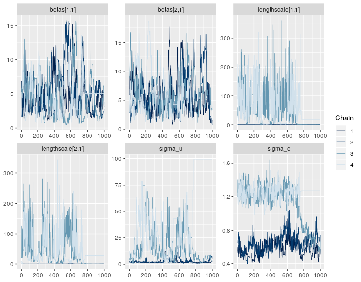
You can make the sampler more effective (less correlated) by increasing the number of leapfrog steps, L. Unlike NUTS (Stan’s default sampler), the HMC algorithm in greta doesn’t tune L, so the user has to specify it. The default value (uniformly sampling L between 5 and 10) works well for models with simple geometry, but probably needs to be increased here. Try:

draws1 <- mcmc(
  m1,
  hmc(Lmin = 20, Lmax = 25),
  one_by_one = TRUE
)

Note that more leapfrog steps implies more evaluations of the posterior density and its gradient, so will take longer to run. Try doubling Lmin and setting Lmax = Lmin + 5, until you get a good trade-off between speed and number of effective samples (see coda::effectiveSize()), the number of effective samples per second is probably the metric you want to look at.

It’s annoying to have to do this tuning for models like this. There’s a development branch of greta that implements NUTS (using a development version of tensorflow probability), though for annoying computational reasons it’s less effective than HMC on less-complicated models. I have a plan to implement tuning of this parameter during warmup, but it’s not trivial and not very high on my to do list. A simple thing we could do quickly (after NUTS is ready to be released in greta) is implement a self-tuning HMC that runs NUTS during warmup, records the distribution of leapfrog steps it takes, then uses that number of leapfrog steps during sampling with vanilla HMC. But manual tuning of L is the most practical solution for now.

BTW, I gave the experimental NUTS sampler a go on this model, and it didn’t do quite as well as vanilla HMC with the L parameters I suggested above.

Option 2. marginalise the intercept

The ML approach to Gaussian processes has some nice features, like the ability to create new kernels by adding and multiplying other kernels. Ie. adding functions together, which implies adding together the resulting variance covariance matrices. See the kernel cookbook for some nice illustrations and explanations.

greta.gp supports this approach to designing GP kernels, so you can define something crazy - like a linear regression with (smoothly) temporally-varying coefficients, plus a spatial random effect - in 5 lines:

n <- 100
x <- cbind(temp = rnorm(n),
           rain = runif(10),
           time = seq_len(n),
           lat = runif(n),
           lon = runif(n))

environmental <- bias(1) + linear(c(5, 5), columns = 1:2)
temporal <- expo(100, 1, columns = 3)
spatial <-   mat32(c(3, 3), 1, columns = c(4:5))
K <- environmental * temporal + spatial
eta <- gp(x, K)

you can also pull out the separate components of this GP, by projecting it using only one of the component kernels

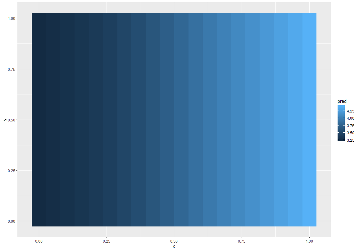
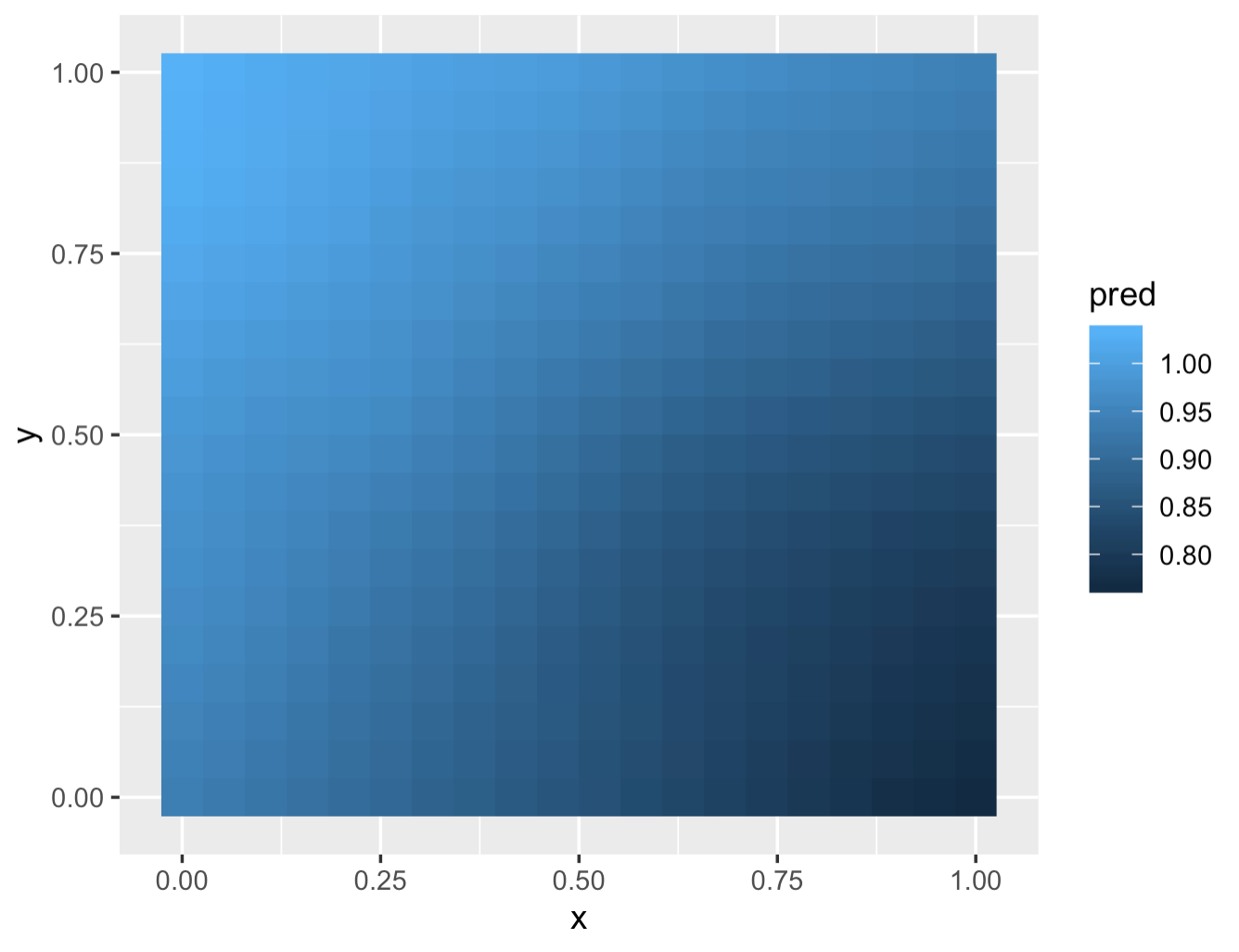
eta_time <- project(eta, x, temporal)

E.g. to fit a model (in this case just the prior) and plot just the temporal effects (which gets multiplied by the environmental linear model) you would do:

m <- model(eta)
draws <- mcmc(m)

eta_time_draws <- calculate(eta_time, draws)
eta_sim <- as.matrix(eta_time_draws)[100, ]
plot(eta_sim ~ x[, "time"], type = "l")

Sorry, that got a bit involved and off topic. Been a while since I played with compositional GPs and got excited.

The interesting thing here though is if you represent an intercept (with normal prior) in the GP ( via the bias() kernel above), it marginalises that parameter. The intercept is a priori Gaussian, and the GP results are a priori Gaussian, so it can combine their variances to get a Gaussian distribution over their sum. That means you don’t need to explicitly model beta_0 at all, it’s taken care of by the GP. You can do:

# beta_0 <- normal(0, 5)
sigma_e <- cauchy(0, 1, truncation = c(0, Inf))
sigma_u <- cauchy(0, 1, truncation = c(0, Inf))
lengthscale <- normal(0, 10, truncation = c(0, Inf))

k1 <- mat32(lengthscale, sigma_u ^ 2)
k2 <- bias(25)  # pass in the prior variance on beta_0 (5 ^ 2)
K <- k1 + k2
f_gp <- gp(pts, K, tol = 1e-6)
f <- f_gp  # + beta_0

distribution(y1) <- normal(f, sigma_e)

m1 <- model(lengthscale, sigma_u)
draws1 <- mcmc(m1, one_by_one = TRUE)

This samples much more nicely, because the geometry is less wacky. You can do the same trick for linear components in the model with the linear kernel.
To extract samples of beta_0 you can do:

beta_0 <- project(f, pts, k2)[1]
beta_0_draws <- calculate(beta_0, draws1)

GPs are magical.

Option 3. Do both.

Using the bias kernel approach, and increasing L a bit would probably be a good idea

1 Like

Wow, thanks a lot @nick for this very detailed answer, it’ll take me some time to digest it (especially the marginalizing part), but I’ll come back shortly with some news on my exploring journey in the magical GP world.

Haha, yep. If only I could write papers one forum response at a time, I’d be much more productive :rofl:

Ok, this is all pretty new and exciting for me. I tried to explore this a bit closer to the model I have in mind. And I have a couple of questions. But first the code I used:

  1. Simulate some data [inspired by your code above]:
n <- 100
x <- data.frame(temp = rnorm(n),
            rain = runif(10),
            lat = runif(n),
            lon = runif(n))
dmat <- as.matrix(dist(x[,c("lon","lat")]))
mu <- 10 + 2 * x$temp - 3 * x$rain
sigma2e <- 0.3
sigma2u <- 2
lengthscale <- 1/7

mcor <- matern32(dmat, lengthscale)
mcov <- sigma2e * diag(nrow(mcor)) + mcor * sigma2u

R <- chol(mcov)
x$y1 <- mu + drop(crossprod(R, rnorm(n)))

The idea is that we want to model the effect of temp and rain with some spatial dependency.

  1. Define all relevant greta-objects and fit the model:
betas <- normal(0, 5, dim = 2) # regression params
lengthscale <- normal(0, 100, truncation = c(0, Inf), dim = 2) # param 1 of Matern corr
sigma_u <- cauchy(0, 5, truncation = c(0, Inf)) # param 2 of Matern corr
sigma_e <- cauchy(0, 5, truncation = c(0, Inf)) # residual variance

main_eff <- bias(10) + linear(betas, columns = 1:2)
spatial <- mat32(lengthscale, sigma_u, columns = 3:4)
K <- main_eff + spatial
eta <- gp(x, K)

distribution(x$y1) <- normal(eta, sigma_e)

m1 <- model(betas, lengthscale, sigma_u, sigma_e)
draws1 <- mcmc(m1, one_by_one = TRUE, hmc(Lmin = 15, Lmax = 20))

I do get quite some awful-looking traceplots:

So some questions:

  • What am I doing wrong?
  • In the crazy example above (time-varying environmental effect with space), you model only the GP (the object eta) and then use project to pull out the relevant infos. Is this better than modelling the hyperparameter of the GP (beta, lengthscale, sigma_u)?
  • How to combine the lengthscale parameter of the two dimensions? In the first examples in this thread we started with one lengthscale parameter for the matern correlation and now with the new formulation we have to pass two. I’d like to plot the expected correlation vs distance between points and am not sure how to do it from two lengthscale parameters.

I start to feel the magic.

Quick answers as I’m on my phone:

  1. You passed the betas to linear(), but it wants the prior variances (25). It thinks you have negative variances, so imagine that’s part of the problem!
  2. I was just being brief. You should definitely model the hyperparameters! You may want to put a bit more prior information in there though.
  3. Just create one lengthscale and replicate it, so: l <- normal(0, 100, truncation = c(0, Inf)) and mat32(c(l, l), ...)

Thanks for your swift answer, applying your suggestions did the charm, I know have nice looking traceplot and good gelman.diag output. I’ll continue my journey to pull out all the needed infos from the fitted model.

Thanks for your patience!

1 Like

Ok, the spatial models on simulated data now fits nicely but when I try to extract the estimated spatial field I get weird results: predicted values only vary along one dimension …

The code I used:

# a function to compute matern correlation
matern32 <- function (distances, lengthscale) {
  a <- sqrt(3 * distances ^ 2) / lengthscale
  (1 + a) * exp(-a)
}

n <- 100
xy <- data.frame(x = runif(n),
                 y = runif(n))

dmat <- as.matrix(dist(xy))
sigma2u <- 1
lengthscale <- 7
sigma2e <- 1
beta0 <- 10

mcor <- matern32(dmat, lengthscale / 7)
mcov <- sigma2e * diag(nrow(mcor)) + mcor * sigma2u

R <- chol(mcov)
xy$y1 <- beta0 + drop(crossprod(R, rnorm(n)))

# greta modeling
sigma_u <- cauchy(0, 5, truncation = c(0, Inf))
sigma_e <- cauchy(0, 5, truncation = c(0, Inf))
length_scale <- normal(0, 10, truncation = c(0, Inf))

spatial <- mat32(length_scale, sigma_u ^ 2)
main_eff <- bias(25)
K <- spatial + main_eff
f_gp <- gp(xy, K, tol = 1e-9)

distribution(xy$y1) <- normal(f_gp, sigma_e)

m1 <- model(length_scale, sigma_u, sigma_e)
draws1 <- mcmc(m1, one_by_one = TRUE, hmc(Lmin = 15, Lmax = 20))

# get spatial at new point
xy_new <- expand.grid(x = seq(0, 1, length.out = 20),
                      y = seq(0, 1, length.out = 20))

f_spat_proj <- project(f_gp, xy_new, spatial)
f_spat_draws <- calculate(f_spat_proj, draws1)
f_spat_m <- colMeans(as.matrix(f_spat_draws))
xy_new$pred <- f_spat_m

ggplot(xy_new, aes(x = x, y = y, fill = pred)) +
  geom_raster()

Which is not what I would expect, if we check the original point to see what spatial patterns there is there:

# compare to y1
ggplot(xy, aes(x = x, y = y, color = y1)) +
  geom_point() +
  scale_color_continuous(low = "orange", high = "green") +
  theme_light()

What am I doing wrong?

Your code doesn’t run for me - it errors because you added the response values to xy and passed that in as the space of the GP. I’m guessing that was not how you ran it when you got these results, but you added that in to help with plotting, so I changed it to:

y1 <- beta0 + drop(crossprod(R, rnorm(n)))

and then:

distribution(y1) <- normal(f_gp, sigma_e)

Then I get the same result as you.


I think the issue here is that you only passed in one lengthscale to greta.gp::mat32, which it interprets as meaning only the first column in the matrix (the x axis) is to be modelled. greta.gp’s matern 32 is non-isotropic by default, so it expects a vector of lengthscales. If you want an isotropic version, you can do:

length_scales <- c(length_scale, length_scale)
spatial <- mat32(length_scales, sigma_u ^ 2)

I then get something like this:

I hadn’t realised that it was silently ignoring axes for which no lengthscale was provided, and that documentation about the argument is vague. I’ll open an issue about this now - we should add a warning or an assertion to catch this unexpected behaviour.

I am starting to fiddle with spatio-temporal models using greta.gp and am encountering the issue that I get a lot (100%) of bad propositions during warmup and sampling.

Here is the code used:

# define hyper-parameter priors
lengthscale_spat <- normal(1, 2, truncation = c(0, 10))
lengthscale_temp <- normal(0, 5, truncation = c(0, 10))
sigma_spat <- cauchy(2, 2, truncation = c(0, 10))
sigma_temp <- cauchy(0, 1, truncation = c(0, 10))
sigma_bias <- cauchy(0, 1, truncation = c(0, 10))

# define the GP
spatial <- mat32(c(lengthscale_spat, lengthscale_spat), sigma_spat ^ 2, columns = 1:2)
temporal <- expo(lengthscale_temp, sigma_temp ^ 2, columns = 3)
intercept <- bias(sigma_bias)

K <- intercept + spatial * temporal

f_gp <- gp(dat[,c("x", "y", "time")], K, tol = 1e-6)

# the response to be modelled
y <- as_data(dat$count)

distribution(y) <- poisson(exp(f_gp))

m_prior <- model(lengthscale_spat, lengthscale_temp,
                 sigma_spat, sigma_temp, sigma_bias)

# sample from the model
drr <- mcmc(m_prior, one_by_one = TRUE, hmc(Lmin = 20, Lmax = 30))

The object dat is a dataframe with 4 columns (x, y, time, count) obtained from simulated data.

Is there something wrong?

I tried to look at:

calculate(y, list(lengthscale_spat = 1,
lengthscale_temp = 1,
sigma_spat = 1,
sigma_temp = 1,
sigma_bias = 1))

As mentioned in the online documentation but I always get the same values out if I change the hyperparameters. Is this what is causing the problem (flat likelihood surface)?

Thanks in advance.

calculate() would just be giving you back the data values of y with these inputs. If you want to simulate values of y you can install the latest GitHub version of greta and do:

calculate(y, nsim = 10)

to get 10 simulations. Or to fix values for hyperparameters e.g.:

calculate(y, values = list(lengthscale_spat = 1), nsim = 10)

The online documentation refers to the version of greta that is on CRAN, so refer to the installed docs for the development version.

I just had a play with this on some fake data (so YMMV) but it looked like switching the temporal kernel to mat32 removed all the bad samples. Not sure why that would be or whether that’s your issue…