How to use LKJ prior?

[Jakob]

Hi everyone,

I am trying to include an LKJ prior in a network model with random sender and receiver effects. However, naively applying the decomposition of the covariance matrix and placing the LKJ prior on the correlation matrix as e.g. documented in the Stan manual (see below) throws tensorflow errors about numerical issues.

tau_a = exponential(.5)
tau_b = exponential(.5)
tau_diag = greta_array(c(tau_a, 0, 0, tau_b), dim = c(2,2))
Omega = lkj_correlation(3, 2)
Sigma_ab = tau_diag %*% Omega %*% tau_diag

ab = multivariate_normal(mean = t(c(0,0)), Sigma = Sigma, dimension = 2, n_realisations = N)

It would be awesome if someone had a simple working example on including an LKJ prior.

Thanks and all the best,
Jakob

[nick]

Hi Jakob,

Thanks for asking this question. It’s one of those cases where there are some handy numerical tricks to speed things up, but I don’t think they’ve been documented anywhere for greta (though this came up in an old, closed GitHub issue https://github.com/greta-dev/greta/issues/281). Here are a few things to consider:

bad proposals

You probably already saw this, but you can handle numerical issues like this failed Cholesky decomposition as bad proposals (divergent transitions in Stan terminology) by setting one_by_one = TRUE in the call to mcmc. Though you don’t want to have many (maybe no more than 1%?) bad samples during the sampling phase as it can lead to biased inferences. Sampling from the prior above gives me bad proposals during sampling, so we need to do something else.

only the diagonal

This won’t actually help with the Cholesky decomposition issue, but it helps with thinking about the next step. In Stan, it’s recommended to use quad_form_diag() using a vector of diagonal elements, rather than the naive matrix multiplies. This skips some multiplications by zero, which makes little difference with a matrix of dimension 2, but can make a big difference as the matrix increases in size. You can do something similar in greta like this (I tidied up a couple of other little things and made it work with generic matrix dimension):

# a not particularly fast version of quad_form_diag, but faster than the matrix
# multiplies for large matrices
quad_form_diag <- function (mat, vec) {
  mat <- sweep(mat, 1, vec, "*")
  sweep(mat, 2, vec, "*")
}

M <- 2
N <- 10
tau <- exponential(0.5, dim = M)
Omega <- lkj_correlation(3, M)
Sigma <- quad_form_diag(Omega, tau)
ab <- multivariate_normal(
  mean = zeros(1, M),
  Sigma = Sigma,
  dimension = M,
  n_realisations = N
)

I’m not planning to include this quad_form_diag() function in greta, because a) It’s not needed when you propagate the Cholesky factors in the next step, and b) I’m hoping this type of operation can soon be automatically detected and done internally - something I’ll talk about at the end.

propagating the Cholesky factors

When greta samples the parameters for Omega, it actually works with the Cholesky factor of the matrix, to get around the symmetry constraint of the matrix. I.e. it samples a matrix U and then forms \Omega = U' U:

Omega <- t(Omega_U) %*% Omega_U

Note: R uses the upper triangular matrix, but you’ll more commonly see the lower triangular matrix L = U' in discussions of Cholesky factorisation.

multivariate_normal() also requires the Cholesky factor of Sigma to compute the density, which it usually obtains by doing a Cholesky decomposition on Sigma. This operation is susceptible to numerical under/overflow, so can fail for some values of the parameters - which is what the errors are about. But if we can get the Cholesky factor of Sigma without doing this decomposition, we can avoid those errors. In fact, the Cholesky factor of Sigma can be computed from the Cholesky factor of Omega and the vector of standard deviations tau, as:

Sigma_U = sweep(Omega_U, 2, tau, '*')

This is the same trick the Stan manual suggests, using diag_pre_multiply() on the vector of standard deviations and the Cholesky factor of the correlation matrix.

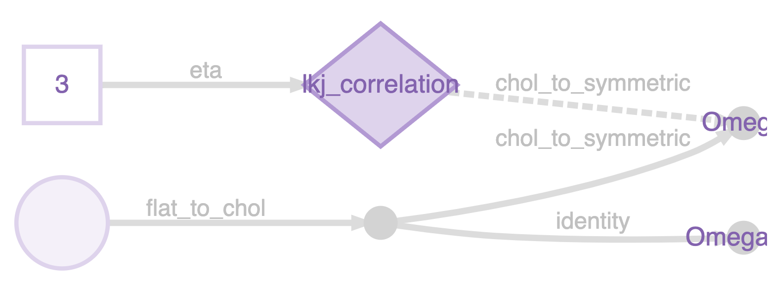
To do this you need Omega_U. The way to do this in greta is just to do: Omega_U <- chol(Omega). greta has an internal mechanism (representations) to skip operations like this when the result is already known. Instead of doing a Cholesky decomposition on Omega, it just grabs the Cholesky factor that it was working with already, and uses that. You can see this if you plot the model:

Omega <- lkj_correlation(3, M)
Omega_U <- chol(Omega)
m <- model(Omega_U)
plot(m)

The nameless variable in the bottom left is a vector-veersion of the Cholesky factor, it’s reshaped into a matrix, and then converted into the symmetric matrix Omega (which is the target of the LKJ distribiution), using internal functions flat_to_chol() and chol_to_symmetric(). But Omega_U is just a copy of the Cholesky factor, no need to decompose it.

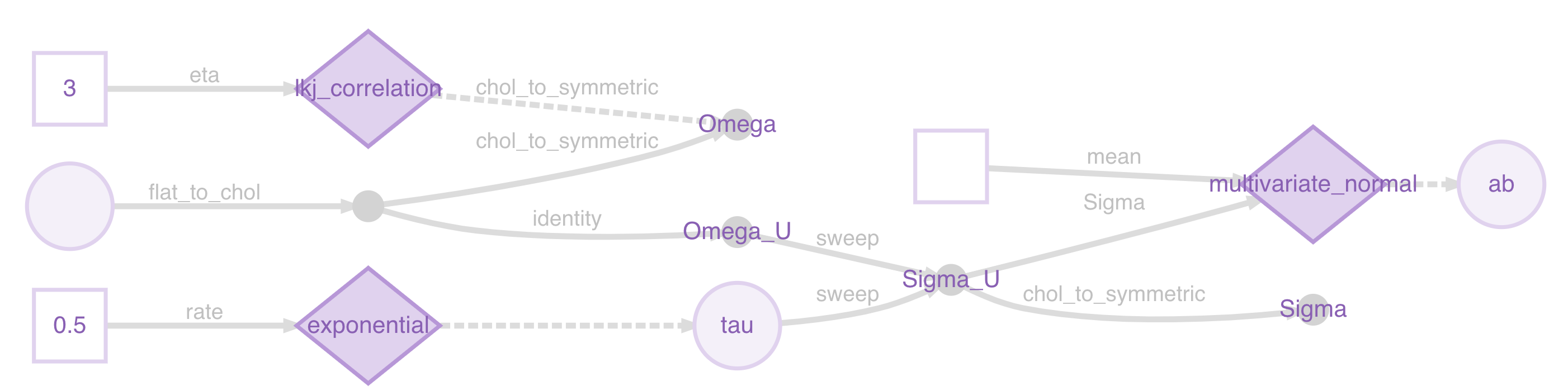
So we can get to Sigma_U without doing a Cholesky decomposition, and then use an internal greta function to turn Sigma_U into Sigma and pass it into multivariate normal. The function chol_to_symmetric() keeps track of the fact that Sigma has a Cholesky factor representation, so that we don’t need a Cholesky decomposition at any point:

chol_to_symmetric <- .internals$utils$greta_array_operations$chol_to_symmetric
M <- 2
N <- 10
tau <- exponential(0.5, dim = M)
Omega <- lkj_correlation(3, M)
Omega_U <- chol(Omega)
Sigma_U <- sweep(Omega_U, 2, tau, "*")
Sigma <- chol_to_symmetric(Sigma_U)
ab <- multivariate_normal(
  mean = zeros(1, M),
  Sigma = Sigma,
  dimension = M,
  n_realisations = N
)

A plot might make this clearer:

m <- model(ab)
plot(m)

You can see the representations being used to pass the Cholesky factors instead of the symmetric matrices at two points.

This still hits an occasional (but much rarer) numerical issue with a matrix solve in computing multivariate normal, but that’s taken care of by one_by_one = TRUE.

whitening decomposition

The above code should work well in a model when the multivariate normal variables are observed, rather than being unknown variables. I.e. when doing this:

distribution(y) <- multivariate_normal(
  mean = zeros(1, M),
  Sigma = Sigma,
  dimension = M,
  n_realisations = N
)

But when ab is an unknown parameter in the model it’s possible to improve sampling again by a ‘whitening’ decomposition (whitening as in removing correlation from; akin to converting to white-noise signal), which is like a multivariate version of hierarchical decentring. This is also mentioned in the Stan manual: https://mc-stan.org/docs/2_18/stan-users-guide/multivariate-hierarchical-priors-section.html

The complete code for this is:

M <- 2
N <- 10
tau <- exponential(0.5, dim = M)
Omega <- lkj_correlation(3, M)
Omega_U <- chol(Omega)
Sigma_U <- sweep(Omega_U, 2, tau, "*")
z <- normal(0, 1, dim = c(N, M))
ab <- z %*% Sigma_U

This samples well, and has no numerical issues when I run it.

future plans

One of the design principles of greta is that the user shouldn’t have to think about this sort of computational and numerical issue when modelling. For relatively common scenarios like this it should just work. That’s why the representations mechanism is there, so that we can use numerical tricks when available. greta doesn’t have both a poisson and a poisson_log distribution like Stan (the latter for working with the log of the rate parameter, for numerical stability) - greta just has poisson() and uses the log representation when it’s available.

Ultimately, I’d like for greta to be able to do that for more complex sets of operations, like in this case. Then the user could just write the naive code like in your example, and greta would handle all the tricks: the diagonalisation; the efficient diagonal multiplication; the propagation of Cholesky factors through the matrix multiplication; and the whitening decomposition if (and only if) the resulting greta array is used as a parameter, not a distribution over data. That quite technically tricky though, so will require a bit of thinking and refactoring.

example model

If someone reading this would like to contribute to greta, adding this last bit of code as an example model on the website would be really helpful! You can find instructions to do that here: https://github.com/greta-dev/greta/blob/master/.EDIT_WEBSITE.md#adding-example-models

[Jakob]

Hi Nick,

thanks a lot for the comprehensive answer, that clarified a lot! The non-centered / whitening decomposition variant works like a charm.

I don’t really have any experience working with GitHub and pkgdown, but I agree that it would be very helpful to have the example on the website as it arguably represents a major use case, e.g. in the social sciences.

All the best and thanks again
Jakob

[nick]

Two quick updates for anyone reading this:

In the dev version (master on GitHub) chol_to_symmetric() is called chol2symm() and is exported as part of greta, so doesn’t need to be fetched as an internal.

@lionel68 added an example “Random intercept-slope model (with correlated effects)” based on this: https://greta-stats.org/articles/example_models.html#common-models

[lzachmann]

Hey Nick, I was wondering if you might be able to share any insights you might have as to how the fixed effect coefficients (as distinct from the additive random effects, or combined fixed + random effects) can be drawn out of the model seen in the ‘Random intercept-slope model (with correlated effects)’ example. Although we’re really interested in the performance gains we might get with that whitening approach, it’s not very clear how we can separate the fixed and random effect components in such a model (though admittedly this is probably because I’m not entirely tracking all of the transformations you are applying to the correlation and covariance matrices). Here’s the sort of thing we do have working, following some of the logic above (where beta_mu is an M-length vector of fixed effect coefficients):

Sigma <- greta:::chol2symm(Sigma_U)
eps <- multivariate_normal(mean = zeros(1, M),
                           Sigma = Sigma,
                           dimension = M,
                           n_realisations = J)
ab <- sweep(eps, 2, beta_mu, "+")

# the linear predictor
mu <- rowSums(ab[d$j, ] * X)

I’ve thrown some code up as a snippet here that shows how we’ve been able to recover the generating values in a simulation without that whitening approach, in case it’s easier to pick at a self-contained example.

[lionel68]

Hi Izachmann,

Am no expert but here are my two cents:

In the non-centered parametrization we have: mu + L * z, where mu is the mean vector, L is the Cholesky factorization of the covariance matrix and z is a standard normal deviate. So what I would do is something like:

# priors on fixed effect coefficients
beta_mu <- normal(0, 10, dim = M)
# broadcast beta_mu to the same dimension as Sigma_U
beta_mu_mat <- greta_array(beta_mu[rep(1:M, each = N)], dim = c(N, M))
...
# equivalent to: ab ~ multi_normal(beta_mu, Sigma_U)
ab <- beta_mu_mat + z %*% Sigma_U 

I tried it out for your snippet and got similar results even if the posterior samples from the approach without the whitening looked better …

Hope this helps,
Lionel

[lzachmann]

Thanks Lionel! And sorry for such a slow reply. Makes a lot of sense at first glance. I’ll give this a shot here in the few weeks. If I’m not back here pestering everybody by then you can assume this solution works! Thanks so much!