Sparse matrix format for count and binary data & setting dtype of tensors

Hello,

I am working on factor analysis model using greta on large count and binary matrices where most values are zero. I know it is possible to convert R Matrix dgCMatrix format to numpy sparse arrays with reticulate. So, I am wondering if it is straightforward to add support for sparse matrices in greta::as_data.

Also on the topic of large data, in the current version is it possible to change the dtype of tensor objects from float64 to float32 or from int64 to int32/int16 to reduce memory footprint of the data and large parameter tensors?

Thanks a lot,

Vitalii

Unfortunately that’s not possible yet. We’re hoping to add support for sparse greta arrays in the future, but it probably won’t be for a while.

Tensorflow doesn’t have great sparse matrix support (not as good as numpy unfortunately), but it can do an efficient matrix multiplication between a dense and a sparse matrix. If this efficiency is important for your model, and you don’t mind digging a little deeper into greta’s internals, I could probably help you to put together a custom greta operation to do this efficiently. What is the operation exactly?

You can switch to single precision easily enough with the precision argument to greta::model(). That only does floats though, greta doesn’t explicitly handle integer greta arrays at the moment.

Thanks for your explanation. I do not mind digging deeper into greta’s internals especially if that’s faster than rewriting my model directly in tensorflow or pytorch.
Without going into too much detail, I need to multiply a dense matrix of parameters by a sparse matrix of data c %*% data and then define poisson distribution over a sparse matrix of data distribution(data) = poisson(mu). This operation is done only once in the model so my main reason for using the sparse matrix format is data size ~5000 * 20000 (dimensions*data points) and can be even larger. So, would it possible to define custom operation for sparse data rather than parameters?

Another way to address my memory problem is to supply less data points in each tensorflow batch (e.g. 20 batches of 1000 points). As far as I understand, the batch size currently is all of the data to enable your way of doing MCMC. Would it be possible to change the batch size at least for likelihood/posterior optimisation with opt()?

1 Like

I would also be interested in a custom greta operation to matrix multiply a dense matrix with a sparse one.If you do end up working it out @vitaliikl, I would love to see the code. On the other hand if you decide not to do it, I may want to give it a try myself, so let me know.

Also, the idea of using minibatches in greta would be really awesome if it could be made to work! It would make possible probabilistic modelling for really truly massive datasets. I’ve seen some interesting papers recently suggesting that stochastic gradient descent can approximate the Bayesian posterior (e.g. the Averaged Stochastic Gradient Sampler https://arxiv.org/abs/1704.04289; goes over my head a little, but trying to work through it because it sounds pretty useful and cool.)

1 Like

I will look into this because I need it for several projects but not a priority for the next 2 weeks.

Oh, yes that would be very useful. Apparently Averaged Stochastic Gradient Sampler is already widely used but I do not see support for it in either tensorflow-probability or pytorch. Support for standard minibatch approach would be very useful in general - not only for massive datasets - I have seen some examples where minibatches improve training compared to full dataset.

I was just writing out the steps to adding this new function, then figured it would be easier to just have a go at implementing it myself. In doing so, I found out that tensorflow’s SparseTensor format doesn’t work with a tensorflow feature called batching, which is essential to how greta works (because of how tensorflow probability does MCMC). Annoyingly that means we can’t use that with greta without some gymnastics. More details follow…

Essentially, a 2D (matrix) greta array with dimension n x m corresponds to a 3D tensor with dimension k x n x m. The first k dimension is the ‘batch’ dimension and is used to simultaneously do inference on multiple MCMC chains, and to make calculate() fast with lots of posterior samples. The tf$sparse$matmul() function can’t automatically handle a batch dimension (most operations on tensors can). However it should be possible to write tensorflow code that reshapes the k x m x n array into a km x n or a m x kn matrix, does the matrix multiply and then reshapes the result back to a 3D array with first dimension of size k.
There’s an open tensorflow issue with some python tensorflow code snippets to do this, which would be a good place to start.


Note that there is another option for sparse matrix multiplication, which is to use tf$matmul(..., b_is_sparse = TRUE). That takes a standard dense tensor as input, not a SparseTensor. It then looks up the 0s. It similarly requires the dense matrix to be 2D, as well as being single precision. So not much to gain in terms of ease of implementation. This page says:

Deciding when to use sparse_tensor_dense_matmul vs. matmul(a_is_sparse=True):

There are a number of questions to ask in the decision process, including:

  • Will the SparseTensor A fit in memory if densified?
  • Is the column count of the product large (>> 1)?
  • Is the density of A larger than approximately 15%?

If the answer to several of these questions is yes, consider converting the SparseTensor to a dense one and > using tf.matmul with a_is_sparse=True.

1 Like

Yes, minibatching the data and some of those subsampling MCMC algorithms would be awesome. It’s not currently implemented, but it has been on the to do list for a long time. There’s a question of how to implement a nice user interface to it, given we need to know all the greta array dimensions when constructing the model.

The easiest option would be to have the user define the model with a single minibatch of the data, then pass in a list of minibatches (or more likely a function to return minibatches on demand) to the inference algorithm. So that interface might look something like this (note this will not work as there is no batch_fun argument to opt, it’s just what the interface could look like):

# full dataset size
n <- 100
k <- 3
X <- matrix(rnorm(n * k), n, k)
y <- rnorm(n)

# user-defined minibatching function (this could load minibatches from disk,
# rather than needing them to be defined in memory, or we could make use of TF's
# functionality for queuing batches)
get_minibatch <- function (size = 10) {
  idx <- sample.int(n, size)
  list(X = X[idx, ], y = y[idx])
}

# use a single minibatch to set up the model with the correct dimensions
mini <- get_minibatch() 

library(greta)
beta <- normal(0, 10, dim = k)
sd <- normal(0, 1, truncation = c(0, Inf))
mu <- mini$X %*% beta
distribution(mini$y) <- normal(mu, sd)

m <- model(beta, sd)

# when running inferencem, use the minibatch function to get a different
# minibatch on each iteration
o <- opt(m, batch_fun = get_minibatch)

That should be straightforward to implement, but potentially limiting in that the minibatches would always have to be the same size. An alternative would be to do a fundamental rewrite of greta so that greta arrays can have unknown dimensions, (perhaps with some sort of placeholder dimension so we can do checking). This seems like it would be confusing though.

Comments on the above interface idea would be welcome!

That led me down a rabbit hole. Here’s a hacked- together implementation of opt() with minibatches, followed by a comparison on logistic regression. I have no idea what I’m doing when it comes to tuning stochastic optimisers, so I’m sure the comparison could be much better.

Shouldn’t be too hard to wrap this into the next release of greta, though I’d appreciate feedback on this approach before then!

opt <- function (model,
                 optimiser = bfgs(),
                 max_iterations = 100,
                 tolerance = 1e-06,
                 initial_values = initials(),
                 adjust = TRUE,
                 hessian = FALSE,
                 batch_fun = NULL) {
  
  prep_initials <- greta:::prep_initials
  
  # if there's a batch function, mess with the model, and later with the optimiser
  if (!is.null(batch_fun)) {
    
    if (optimiser$class$classname != "tf_optimiser") {
      stop ("minibatching is only compatible with tensorflow optimisers, ",
            "not scipy optimisers", call. = FALSE)
    }
   
    # find tensors corresponding to the minibatched data
    example_batch <- batch_fun()
    batched_greta_array_names <- names(example_batch)
    batched_greta_arrays <- lapply(
      batched_greta_array_names,
      get,
      envir = parent.frame()
    )
    
    tf_names <- vapply(
      batched_greta_arrays,
      function (ga) {
        model$dag$tf_name(greta:::get_node(ga))
      },
      FUN.VALUE = character(1)
    )
    
    # replace the build_feed_dict function with a version that draws minibatches each time
    build_feed_dict <- function (dict_list = list(),
                                 data_list = self$tf_environment$data_list) {
      
      tfe <- self$tf_environment
      
      # replace appropriate elements of data_list with minibatches
      batch <- batch_fun()
      names(batch) <- tf_names
      for (name in tf_names) {
        data_list[[name]][] <- batch[[name]]
      }
      
      # put the list in the environment temporarily
      tfe$dict_list <- c(dict_list, data_list)
      on.exit(rm("dict_list", envir = tfe))
      
      # roll into a dict in the tf environment
      self$tf_run(feed_dict <- do.call(dict, dict_list))
    }
    
    # fix the environment of this function and put required information in there
    dag_env <- model$dag$.__enclos_env__
    environment(build_feed_dict) <- dag_env
    dag_env$batch_fun <- batch_fun
    dag_env$tf_names <- tf_names
    
    # replace the functions with these new ones
    unlockBinding("build_feed_dict", env = model$dag)
    model$dag$build_feed_dict <- build_feed_dict
    lockBinding("build_feed_dict", env = model$dag)
     
  }
  
  # check initial values. Can up the number of chains in the future to handle
  # random restarts
  initial_values_list <- prep_initials(initial_values, 1, model$dag)
  
  # create R6 object of the right type
  object <- optimiser$class$new(initial_values = initial_values_list[1],
                                model = model,
                                name = optimiser$name,
                                method = optimiser$method,
                                parameters = optimiser$parameters,
                                other_args = optimiser$other_args,
                                max_iterations = max_iterations,
                                tolerance = tolerance,
                                adjust = adjust)
  
  # if there's a batch function, mess with the minimiser to change batch at
  # every iteration
  if (!is.null(batch_fun)) {
    
    run_minimiser <- function() {
      
      self$set_inits()
      
      while (self$it < self$max_iterations &
             self$diff > self$tolerance) {
        self$it <- self$it + 1
        
        self$model$dag$build_feed_dict()
        
        self$model$dag$tf_sess_run(train)
        if (self$adjust) {
          obj <- self$model$dag$tf_sess_run(optimiser_objective_adj)
        } else {
          obj <- self$model$dag$tf_sess_run(optimiser_objective)
        }
        self$diff <- abs(self$old_obj - obj)
        self$old_obj <- obj
      }
      
    }
    
    environment(run_minimiser) <- object$.__enclos_env__
    
    # replace the functions with these new ones
    unlockBinding("run_minimiser", env = object)
    object$run_minimiser <- run_minimiser
    lockBinding("run_minimiser", env = object)
    
  }
  
  # run it and get the outputs
  object$run()
  outputs <- object$return_outputs()
  
  # optionally evaluate the hessians at these parameters (return as hessian for
  # objective function)
  if (hessian) {
    hessians <- model$dag$hessians()
    hessians <- lapply(hessians, `*`, -1)
    outputs$hessian <- hessians
  }
  
  outputs
  
}
# ~~~~~~~~~
# full dataset
set.seed(2019-06-29)
n <- 500000
k <- 50
X_big <- cbind(1, matrix(rnorm(n * k), n, k))
beta_true <- rnorm(k + 1, 0, 0.1)
y_big <- rbinom(n, 1, plogis(X_big %*% beta_true))


library(greta)

# ~~~~~~~~~
# model with all the data
beta <- normal(0, 10, dim = k + 1)
eta <- X_big %*% beta
p <- ilogit(eta)
distribution(y_big) <- bernoulli(p)
m_full <- model(beta)

# ~~~~~~~~~
# model with minibatches

# user-defined minibatching function (this could load minibatches from disk,
# rather than needing them to be defined in memory, or we could make use of TF's
# functionality for queuing batches)
get_minibatch <- function (size = 1000) {
  idx <- sample.int(n, size)
  list(X = X_big[idx, ], y = y_big[idx])
}

# use a single minibatch to set up the model with the correct dimensions. Must
# use as_data here so that the data can be swapped in, and the names of those
# greta arrays must match the names returned by get_minibatch 
mini <- get_minibatch() 
X <- as_data(mini$X)
y <- as_data(mini$y)
beta <- normal(0, 10, dim = k + 1)
eta <- X %*% beta
p <- ilogit(eta)
distribution(y) <- bernoulli(p)
m_mini <- model(beta)

# ~~~~~~~~~

# run the two optimisers and a glm

full_time <- system.time(
  o_full <- opt(m_full)
)

mini_time <- system.time(
  o_mini <- opt(
    m_mini,
    optimiser = adam(learning_rate = 0.01),
    tolerance = 0,
    max_iterations = 100,
    batch_fun = get_minibatch
  )
)

glm_time <- system.time(
  o_glm <- glm(y_big ~ . - 1,
               data = data.frame(X_big),
               family = stats::binomial)
)

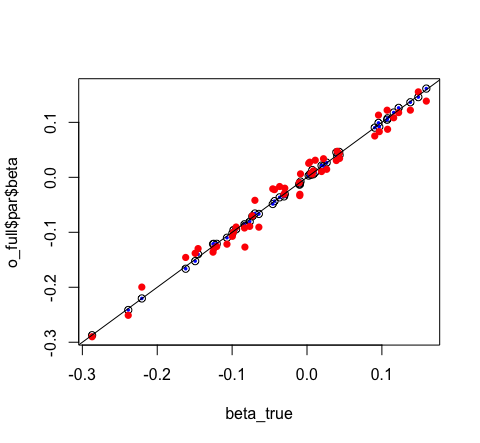
# visually compare them
plot(o_full$par$beta ~ beta_true)
points(o_glm$coefficients ~ beta_true, pch = 16, col = "blue", cex = 0.5)
points(o_mini$par$beta ~ beta_true, pch = 16, col = "red")
abline(0, 1)

comparison

full_time
   user  system elapsed 
 74.351  13.486  41.860 
mini_time
   user  system elapsed 
  2.178   0.203   1.581
glm_time
    user  system elapsed 
  7.757   1.116   8.890 
2 Likes

NB. This is returning the final stat of the minibatched optimiser, rather than averaging over the last n states, which would probably be much more sensible.

Wow, this looks cool! I’m definitely going to give it a try and I will get back to you with feedback. On a related note, have you seen this R package : https://github.com/STOR-i/sgmcmc ?
It also uses tensorflow as its backend, implementing several stochastic gradient MCMC methods. Looks interesting.

Anyway, thanks for putting that work in. I’ll be playing with this code shortly.

Cheers!

@nick Thanks a lot for going into that rabbit hole! Your minibatch opt() function works for me. I think the interface is pretty straightforward. The need to rewrite the model to use minibatch is a bit annoying but it is straightforward to do. If I am not wrong keras guesses tensor dimensions based on batch size/number of batches, but that probably requires some rigidity on how one data point can be defined (e.g. one row of X and y), so your approach is more flexible.

Maybe I am not making sense here, but the current version of minibatch is not compatible with factor analysis. E.i. if I want to have both the variable and data point factors but define the minibatch model than the dimensions of data point factors will be dim(Z) = c(n_factors, batch_size) rather than c(n_factors, n_data_points). Do you see a solution for this? (if it make sense to do stochastic inference for factor analysis)
That is, is it possible to define which parameters should be updated in each minibatch by swapping in the right part of the parameter matrix (e.g. via get_parameter_minibatch function)? And if yes, do you see a general rather than model-specific implementation of this?

Thanks again and sorry for a slow reply.

This is what I mean by factor analysis model (potentially using more complex priors):

reticulate::use_condaenv("r-tensorflow", conda = "auto", required = TRUE)
library(greta)
library(bayesplot)

# generate data
generate.data <- function(n = 100, p = 5, q = 2, psi = diag(rgamma(p, 1, 1)))
{
  W  <- matrix(rnorm(p * q, 1), p, q)
  Z  <- matrix(rnorm(q * n, 2), q, n)
  WZ <- W %*% Z

  X  <- matrix(0, n, p)
  for (i in seq_len(n)) {
    X[i, ] <- MASS::mvrnorm(1, WZ[, i], psi)
  }

  list(X = X, W = W, Z = Z, psi = psi)
}

n <- 10000
p <- 10
q <- 2
data <- generate.data(n = n, p = p, q = q)
X_full <- data$X

## Define models:

# Full model:
W <- normal(0, 1, dim = c(ncol(X_full), q))
Z <- normal(0, 1, dim = c(q, nrow(X_full)))
psi <- zeros(ncol(X_full), ncol(X_full))
diag(psi) <- inverse_gamma(1, 1, dim = ncol(X_full))

distribution(X_full) <- multivariate_normal(t(W %*% Z), psi)

m_full <- model(W, Z, psi)

# Minibatch model:

# generate minibatch
get_minibatch <- function(n_sam = 100) {
  ind <- sample.int(nrow(X_full), n_sam)
  list(X = X_full[ind,])
}
mini <- get_minibatch()
X = as_data(mini$X)

W <- normal(0, 1, dim = c(ncol(X), q))
Z <- normal(0, 1, dim = c(q, nrow(X)))
psi <- zeros(ncol(X), ncol(X))
diag(psi) <- inverse_gamma(1, 1, dim = ncol(X))

distribution(X) <- multivariate_normal(t(W %*% Z), psi)

m_mini <- model(W, Z, psi)

## Fit both models

time = Sys.time()
res_full = opt(m_full,
              optimiser = adam(learning_rate = 0.1),
              max_iterations = 500,
              tolerance = 1e-4,
              adjust = TRUE,
              hessian = FALSE)
Sys.time() - time
res_full$iterations


time = Sys.time()
res_mini = opt(m_mini,
              optimiser = adam(learning_rate = 0.01),
              max_iterations = 2000,
              tolerance = 1e-4,
              batch_fun = get_minibatch,
              adjust = TRUE,
              hessian = FALSE)
Sys.time() - time
res_mini$iterations

Yeah, that’s a good point. I’m no expert on minibatching and related stochastic gradient approaches, but as I understand it you need to have some set of control parameters that are always in the model. So having a random variable for each observation (like in a factor analysis) is problematic.

If you can get away with inducing some dependence between the factors (in e.g. a spatial- or temporal-factor analysis) then you might be able to model that with some control parameters. I’ve heard of this being done for stochastic gradient inference on Gaussian process models - it fits naturally with sparse Gaussian processes where the GP is modelled with a series of ‘inducing points’ and then projected onto the GP values for the different observations. Because the inducing points are always the same, you can minibatch it.

1 Like

I was going to try implementing the sparse matrix multiplication but I realised that it needs a different greta array data type which is connected to tensorflow sparse tensor underneath. I do not understand R6 objects well enough at this point to implement this sparse data array, especially the one that can be used in distribution(sparse_data) <- normal(mu, sd).

I will have a look at the sparse Gaussian processes, thanks!

Yeah, there’s a fair bit of thinking to be done on API design and architecture to implement sparse greta arrays in a sensible way. It’s a shame there isn’t good support in TensorFlow for these ops.

For defining a likelihood on sparse data, you could do something like this (assuming this sparsity is missingness, not 0s), where non_sparse_idx is either: a two column R matrix of integers giving the row and column numbers of the (non-missing) data; or an R vector of integers giving the cell number of the data:

data_vec <- sparse_data[non_sparse_idx]
mu_vec <- mu[non_sparse_idx]
distribution(data_vec) <- normal(mu_vec, sd)

Doing the operations on sparse greta arrays is harder. The easiest thing if you did want to implement this would be to write tensorflow code for the batched sparse operation, and register that as an op. There’s no need for R6 in that approach, though it still requires the awkward tensorflow stuff, so far from trivial.

Makes sense to use the sparse definition you suggest when sparsity means missing data. I think in my case of gene expression many 0s are 0s.

Now I am a bit confused about operations. c %*% data is the operation I want to define where c is a greta variable and data is data matrix. I thought the operation is only possible if data is converted to greta array with as_data() which means the need for sparse greta array data type.

Right, that’s true if you want to use %*%, which I think would be the best thing in a full greta sparse implementation.

But if you wanted to write your own new op for this specific operation you could. The way I would do it is to create a new R function (that creates an operation greta array) called, say, sparse_matmul(), which would take in a greta array c and a dgCMatrix data. That function could turn only the vector of non-sparse values in data into a greta array, using as_data, and pass in those two greta arrays as the main arguments to greta:::op(), and the rest of the information (locations of non-sparse values, and matrix dimensions) in as R objects, via the operation_args argument to op(). See sweep.greta_array for a similar example.

That would handle things on the greta side, but you’d also need a tensorflow function to pass in to op(), and unfortunately the one in tensorflow won’t work. Hence the awkward reshaping code suggested above.