Spatial model with SPDE in greta

lionel68 · November 1, 2021, 10:32am

A thread on this topic was started for Stan but given that greta is just as cool I decided to have a shot at fitting SPDE spatial models similar to what INLA does but using greta and this article. So this is not using the greta.gp package.

Here is the model code (the data generation code is given at the end of the post):

y <- dat$resp

# the model parameters
mu <- normal(0, 1)
kappa <- lognormal(0, 1) # variance of spatial effect
tau <- gamma(0.1, 0.1) # scale of spatial effect
sigma <- lognormal(0, 1)
z <- normal(0, 1, dim = mesh$n) # std-normal variable for non-centered parametrization

# the precision matrix of the spatial effect
S <- (tau ** 2) * (G[1,,] * kappa ** 4 + G[2,,] * 2 * kappa ** 2 + G[3,,])
# drawing the spatial effect coefficient
beta <- backsolve(chol(S), z)

# the linear predictor
linpred <- mu + A %*% beta
distribution(y) <- normal(linpred, sigma)

# fitting the model
m_g <- model(mu, sigma, tau, kappa)
m_draw <- mcmc(m_g, one_by_one = TRUE)
bayesplot::mcmc_trace(m_draw)
coda::gelman.diag(m_draw)

The resulting draws shows that the chains get sometimes stuck and that the sampling of tau is not optimal:

So to my questions:

Is the model code correct?
How to improve sampling?

Thx in advance for your inputs!

Now the R code to generate the data:

library(rstan)
library(INLA)
library(RandomFields)

dat <- data.frame(x = runif(100),
                  y = runif(100))

spat_field <- raster::raster(RFsimulate(RMmatern(nu=1, var = 1, scale = 0.1),
                         x = seq(0, 1, length.out = 100),
                         y = seq(0, 1, length.out = 100),
                         spConform = FALSE))
dat$resp <- rnorm(100, mean = 1 + raster::extract(spat_field, dat), sd = 1)
bnd <- inla.mesh.segment(matrix(c(0, 0, 1, 0, 1, 1, 0, 1), 4, 2, byrow = TRUE))

# a coarse mesh
mesh <- inla.mesh.2d(max.edge = 0.2,
                     offset = 0,
                     boundary = bnd)

# derive the FEM matrices
fem <- inla.mesh.fem(mesh)
# put the matrices in one object
G <- array(c(as(fem$c1, "matrix"),
             as(fem$g1, "matrix"),
             as(fem$g2, "matrix")),
          dim = c(mesh$n, mesh$n, 3))
G <- aperm(G, c(3, 1, 2))

# derive the projection matrix
A <- inla.spde.make.A(mesh, loc = as.matrix(dat[,c("x", "y")]))
A <- as(A, "matrix")

njtierney · November 4, 2021, 9:25am

Hi @lionel68!

Thanks so much for sharing this,

I just wanted to post my reprex of your results - I’ll check in with Nick G about this, I haven’t done spatial modelling for a little while, but thanks so much for sharing this!

library(rstan)
#> Loading required package: StanHeaders
#> Loading required package: ggplot2
#> rstan (Version 2.21.2, GitRev: 2e1f913d3ca3)
#> For execution on a local, multicore CPU with excess RAM we recommend calling
#> options(mc.cores = parallel::detectCores()).
#> To avoid recompilation of unchanged Stan programs, we recommend calling
#> rstan_options(auto_write = TRUE)
library(INLA)
#> Loading required package: Matrix
#> Loading required package: foreach
#> Loading required package: parallel
#> Loading required package: sp
#> This is INLA_21.05.02 built 2021-05-03 11:17:14 UTC.
#>  - See www.r-inla.org/contact-us for how to get help.
#>  - To enable PARDISO sparse library; see inla.pardiso()
library(RandomFields)
#> Loading required package: RandomFieldsUtils
#> 
#> Attaching package: 'RandomFields'
#> The following object is masked from 'package:RandomFieldsUtils':
#> 
#>     RFoptions
library(greta)
#> 
#> Attaching package: 'greta'
#> The following object is masked from 'package:INLA':
#> 
#>     f
#> The following objects are masked from 'package:Matrix':
#> 
#>     chol2inv, colMeans, colSums, cov2cor, diag, rowMeans, rowSums
#> The following objects are masked from 'package:stats':
#> 
#>     binomial, cov2cor, poisson
#> The following objects are masked from 'package:base':
#> 
#>     %*%, apply, backsolve, beta, chol2inv, colMeans, colSums, diag,
#>     eigen, forwardsolve, gamma, identity, rowMeans, rowSums, sweep,
#>     tapply

dat <- data.frame(x = runif(100),
                  y = runif(100))

spat_field <- raster::raster(RFsimulate(RMmatern(nu=1, var = 1, scale = 0.1),
                                        x = seq(0, 1, length.out = 100),
                                        y = seq(0, 1, length.out = 100),
                                        spConform = FALSE))
dat$resp <- rnorm(100, mean = 1 + raster::extract(spat_field, dat), sd = 1)
bnd <- inla.mesh.segment(matrix(c(0, 0, 1, 0, 1, 1, 0, 1), 4, 2, byrow = TRUE))

# a coarse mesh
mesh <- inla.mesh.2d(max.edge = 0.2,
                     offset = 0,
                     boundary = bnd)

# derive the FEM matrices
fem <- inla.mesh.fem(mesh)
# put the matrices in one object
G <- array(c(as(fem$c1, "matrix"),
             as(fem$g1, "matrix"),
             as(fem$g2, "matrix")),
           dim = c(mesh$n, mesh$n, 3))
G <- aperm(G, c(3, 1, 2))

# derive the projection matrix
A <- inla.spde.make.A(mesh, loc = as.matrix(dat[,c("x", "y")]))
A <- as(A, "matrix")

y <- dat$resp

# the model parameters
mu <- normal(0, 1)
#> ℹ Initialising python and checking dependencies, this may take a moment.
#> ✓ Initialising python and checking dependencies ... done!
#> 
kappa <- lognormal(0, 1) # variance of spatial effect
tau <- gamma(0.1, 0.1) # scale of spatial effect
sigma <- lognormal(0, 1)
z <- normal(0, 1, dim = mesh$n) # std-normal variable for non-centered parametrization

# the precision matrix of the spatial effect
S <- (tau ** 2) * (G[1,,] * kappa ** 4 + G[2,,] * 2 * kappa ** 2 + G[3,,])
# drawing the spatial effect coefficient
beta <- backsolve(chol(S), z)

# the linear predictor
linpred <- mu + A %*% beta
distribution(y) <- normal(linpred, sigma)

# fitting the model
m_g <- model(mu, sigma, tau, kappa)
m_draw <- mcmc(m_g, one_by_one = TRUE)
#> running 4 chains simultaneously on up to 8 cores 

#> warmup 0/1000 \| eta: ?s warmup == 50/1000 \| eta: 2m warmup ==== 100/1000 \| eta: 1m warmup ====== 150/1000 \| eta: 1m \| 5% bad warmup ======== 200/1000 \| eta: 1m \| 4% bad warmup ========== 250/1000 \| eta: 43s \| 4% bad warmup =========== 300/1000 \| eta: 38s \| 5% bad warmup ============= 350/1000 \| eta: 35s \| 5% bad warmup =============== 400/1000 \| eta: 31s \| 5% bad warmup ================= 450/1000 \| eta: 28s \| 7% bad warmup =================== 500/1000 \| eta: 25s \| 6% bad warmup ===================== 550/1000 \| eta: 22s \| 6% bad warmup ======================= 600/1000 \| eta: 19s \| 6% bad warmup ========================= 650/1000 \| eta: 17s \| 6% bad warmup =========================== 700/1000 \| eta: 14s \| 5% bad warmup ============================ 750/1000 \| eta: 12s \| 5% bad warmup ============================== 800/1000 \| eta: 9s \| 5% bad warmup ================================ 850/1000 \| eta: 7s \| 5% bad warmup ================================== 900/1000 \| eta: 4s \| 5% bad warmup ==================================== 950/1000 \| eta: 2s \| 4% bad warmup ====================================== 1000/1000 \| eta: 0s \| 4% bad
#> sampling 0/1000 \| eta: ?s sampling == 50/1000 \| eta: 34s sampling ==== 100/1000 \| eta: 32s sampling ====== 150/1000 \| eta: 30s sampling ======== 200/1000 \| eta: 28s sampling ========== 250/1000 \| eta: 26s sampling =========== 300/1000 \| eta: 24s sampling ============= 350/1000 \| eta: 23s sampling =============== 400/1000 \| eta: 21s \| \<1% bad sampling ================= 450/1000 \| eta: 20s \| \<1% bad sampling =================== 500/1000 \| eta: 18s \| \<1% bad sampling ===================== 550/1000 \| eta: 17s \| \<1% bad sampling ======================= 600/1000 \| eta: 15s \| 1% bad sampling ========================= 650/1000 \| eta: 13s \| 2% bad sampling =========================== 700/1000 \| eta: 11s \| 2% bad sampling ============================ 750/1000 \| eta: 9s \| 2% bad sampling ============================== 800/1000 \| eta: 8s \| 1% bad sampling ================================ 850/1000 \| eta: 6s \| 1% bad sampling ================================== 900/1000 \| eta: 4s \| 1% bad sampling ==================================== 950/1000 \| eta: 2s \| 1% bad sampling ====================================== 1000/1000 \| eta: 0s \| 1% bad

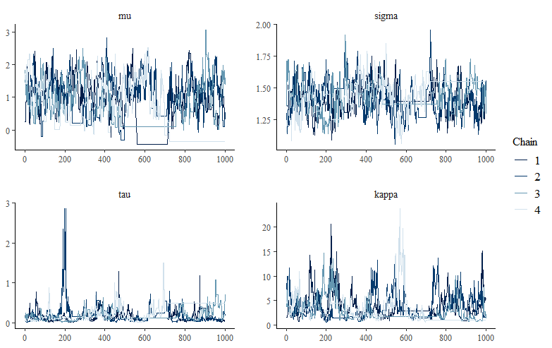
bayesplot::mcmc_trace(m_draw)

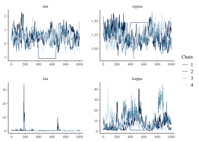
    coda::gelman.diag(m_draw)
    #> Potential scale reduction factors:
    #> 
    #>       Point est. Upper C.I.
    #> mu          1.25       1.70
    #> sigma       1.13       1.37
    #> tau         1.22       1.56
    #> kappa       1.30       1.93
    #> 
    #> Multivariate psrf
    #> 
    #> 1.23

^{Created on 2021-11-04 by the reprex package (v2.0.1)}

Session info

sessioninfo::session_info()
#> ─ Session info ───────────────────────────────────────────────────────────────
#>  setting  value                       
#>  version  R version 4.1.1 (2021-08-10)
#>  os       macOS Big Sur 10.16         
#>  system   x86_64, darwin17.0          
#>  ui       X11                         
#>  language (EN)                        
#>  collate  en_AU.UTF-8                 
#>  ctype    en_AU.UTF-8                 
#>  tz       Australia/Perth             
#>  date     2021-11-04                  
#> 
#> ─ Packages ───────────────────────────────────────────────────────────────────
#>  package           * version    date       lib source        
#>  abind               1.4-5      2016-07-21 [1] CRAN (R 4.1.0)
#>  assertthat          0.2.1      2019-03-21 [1] CRAN (R 4.1.0)
#>  backports           1.2.1      2020-12-09 [1] CRAN (R 4.1.0)
#>  base64enc           0.1-3      2015-07-28 [1] CRAN (R 4.1.0)
#>  bayesplot           1.8.1      2021-06-14 [1] CRAN (R 4.1.0)
#>  callr               3.7.0      2021-04-20 [1] CRAN (R 4.1.0)
#>  cli                 3.1.0      2021-10-27 [1] CRAN (R 4.1.1)
#>  coda                0.19-4     2020-09-30 [1] CRAN (R 4.1.0)
#>  codetools           0.2-18     2020-11-04 [1] CRAN (R 4.1.1)
#>  colorspace          2.0-2      2021-06-24 [1] CRAN (R 4.1.0)
#>  crayon              1.4.1      2021-02-08 [1] CRAN (R 4.1.0)
#>  curl                4.3.2      2021-06-23 [1] CRAN (R 4.1.0)
#>  DBI                 1.1.1      2021-01-15 [1] CRAN (R 4.1.0)
#>  digest              0.6.28     2021-09-23 [1] CRAN (R 4.1.0)
#>  dplyr               1.0.7      2021-06-18 [1] CRAN (R 4.1.0)
#>  ellipsis            0.3.2      2021-04-29 [1] CRAN (R 4.1.0)
#>  evaluate            0.14       2019-05-28 [1] CRAN (R 4.1.0)
#>  fansi               0.5.0      2021-05-25 [1] CRAN (R 4.1.0)
#>  farver              2.1.0      2021-02-28 [1] CRAN (R 4.1.0)
#>  fastmap             1.1.0      2021-01-25 [1] CRAN (R 4.1.0)
#>  foreach           * 1.5.1      2020-10-15 [1] CRAN (R 4.1.0)
#>  fs                  1.5.0      2020-07-31 [1] CRAN (R 4.1.0)
#>  future              1.23.0     2021-10-31 [1] CRAN (R 4.1.1)
#>  generics            0.1.1      2021-10-25 [1] CRAN (R 4.1.0)
#>  ggplot2           * 3.3.5      2021-06-25 [1] CRAN (R 4.1.0)
#>  ggridges            0.5.3      2021-01-08 [1] CRAN (R 4.1.0)
#>  globals             0.14.0     2020-11-22 [1] CRAN (R 4.1.0)
#>  glue                1.4.2      2020-08-27 [1] CRAN (R 4.1.0)
#>  greta             * 0.3.1.9012 2021-11-03 [1] local         
#>  gridExtra           2.3        2017-09-09 [1] CRAN (R 4.1.0)
#>  gtable              0.3.0      2019-03-25 [1] CRAN (R 4.1.0)
#>  here                1.0.1      2020-12-13 [1] CRAN (R 4.1.0)
#>  highr               0.9        2021-04-16 [1] CRAN (R 4.1.0)
#>  hms                 1.1.1      2021-09-26 [1] CRAN (R 4.1.0)
#>  htmltools           0.5.2      2021-08-25 [1] CRAN (R 4.1.0)
#>  httr                1.4.2      2020-07-20 [1] CRAN (R 4.1.0)
#>  INLA              * 21.05.02   2021-05-03 [1] local         
#>  inline              0.3.19     2021-05-31 [1] CRAN (R 4.1.0)
#>  iterators           1.0.13     2020-10-15 [1] CRAN (R 4.1.0)
#>  jsonlite            1.7.2      2020-12-09 [1] CRAN (R 4.1.0)
#>  knitr               1.36       2021-09-29 [1] CRAN (R 4.1.0)
#>  labeling            0.4.2      2020-10-20 [1] CRAN (R 4.1.0)
#>  lattice             0.20-44    2021-05-02 [1] CRAN (R 4.1.1)
#>  lifecycle           1.0.1      2021-09-24 [1] CRAN (R 4.1.0)
#>  listenv             0.8.0      2019-12-05 [1] CRAN (R 4.1.0)
#>  loo                 2.4.1      2020-12-09 [1] CRAN (R 4.1.0)
#>  magrittr            2.0.1      2020-11-17 [1] CRAN (R 4.1.0)
#>  Matrix            * 1.3-4      2021-06-01 [1] CRAN (R 4.1.1)
#>  matrixStats         0.61.0     2021-09-17 [1] CRAN (R 4.1.0)
#>  mime                0.12       2021-09-28 [1] CRAN (R 4.1.0)
#>  munsell             0.5.0      2018-06-12 [1] CRAN (R 4.1.0)
#>  parallelly          1.28.1     2021-09-09 [1] CRAN (R 4.1.0)
#>  pillar              1.6.4      2021-10-18 [1] CRAN (R 4.1.0)
#>  pkgbuild            1.2.0      2020-12-15 [1] CRAN (R 4.1.0)
#>  pkgconfig           2.0.3      2019-09-22 [1] CRAN (R 4.1.0)
#>  plyr                1.8.6      2020-03-03 [1] CRAN (R 4.1.0)
#>  png                 0.1-7      2013-12-03 [1] CRAN (R 4.1.0)
#>  prettyunits         1.1.1      2020-01-24 [1] CRAN (R 4.1.0)
#>  processx            3.5.2      2021-04-30 [1] CRAN (R 4.1.0)
#>  progress            1.2.2      2019-05-16 [1] CRAN (R 4.1.0)
#>  ps                  1.6.0      2021-02-28 [1] CRAN (R 4.1.0)
#>  purrr               0.3.4      2020-04-17 [1] CRAN (R 4.1.0)
#>  R.cache             0.15.0     2021-04-30 [1] CRAN (R 4.1.0)
#>  R.methodsS3         1.8.1      2020-08-26 [1] CRAN (R 4.1.0)
#>  R.oo                1.24.0     2020-08-26 [1] CRAN (R 4.1.0)
#>  R.utils             2.11.0     2021-09-26 [1] CRAN (R 4.1.0)
#>  R6                  2.5.1      2021-08-19 [1] CRAN (R 4.1.0)
#>  RandomFields      * 3.3.8      2020-02-06 [1] CRAN (R 4.1.0)
#>  RandomFieldsUtils * 0.5.4      2021-09-22 [1] CRAN (R 4.1.0)
#>  raster              3.4-13     2021-06-18 [1] CRAN (R 4.1.0)
#>  Rcpp                1.0.7      2021-07-07 [1] CRAN (R 4.1.0)
#>  RcppParallel        5.1.4      2021-05-04 [1] CRAN (R 4.1.0)
#>  reprex              2.0.1      2021-08-05 [1] CRAN (R 4.1.0)
#>  reshape2            1.4.4      2020-04-09 [1] CRAN (R 4.1.0)
#>  reticulate          1.22       2021-09-17 [1] CRAN (R 4.1.0)
#>  rgdal               1.5-27     2021-09-16 [1] CRAN (R 4.1.0)
#>  rlang               0.4.12     2021-10-18 [1] CRAN (R 4.1.0)
#>  rmarkdown           2.11       2021-09-14 [1] CRAN (R 4.1.0)
#>  rprojroot           2.0.2      2020-11-15 [1] CRAN (R 4.1.0)
#>  rstan             * 2.21.2     2020-07-27 [1] CRAN (R 4.1.0)
#>  rstudioapi          0.13       2020-11-12 [1] CRAN (R 4.1.0)
#>  scales              1.1.1      2020-05-11 [1] CRAN (R 4.1.0)
#>  sessioninfo         1.1.1      2018-11-05 [1] CRAN (R 4.1.0)
#>  sp                * 1.4-5      2021-01-10 [1] CRAN (R 4.1.0)
#>  StanHeaders       * 2.21.0-7   2020-12-17 [1] CRAN (R 4.1.0)
#>  stringi             1.7.5      2021-10-04 [1] CRAN (R 4.1.0)
#>  stringr             1.4.0      2019-02-10 [1] CRAN (R 4.1.0)
#>  styler              1.6.2      2021-09-23 [1] CRAN (R 4.1.0)
#>  tensorflow          2.6.0      2021-08-19 [1] CRAN (R 4.1.0)
#>  tfruns              1.5.0      2021-02-26 [1] CRAN (R 4.1.0)
#>  tibble              3.1.5      2021-09-30 [1] CRAN (R 4.1.0)
#>  tidyselect          1.1.1      2021-04-30 [1] CRAN (R 4.1.0)
#>  utf8                1.2.2      2021-07-24 [1] CRAN (R 4.1.0)
#>  V8                  3.4.2      2021-05-01 [1] CRAN (R 4.1.0)
#>  vctrs               0.3.8      2021-04-29 [1] CRAN (R 4.1.0)
#>  whisker             0.4        2019-08-28 [1] CRAN (R 4.1.0)
#>  withr               2.4.2      2021-04-18 [1] CRAN (R 4.1.0)
#>  xfun                0.26       2021-09-14 [1] CRAN (R 4.1.0)
#>  xml2                1.3.2      2020-04-23 [1] CRAN (R 4.1.0)
#>  yaml                2.2.1      2020-02-01 [1] CRAN (R 4.1.0)
#> 
#> [1] /Library/Frameworks/R.framework/Versions/4.1/Resources/library

BertvdVeen · February 3, 2023, 7:43am

Reviving this thread as I am interested in this, @njtierney did you make any progress?

njtierney · February 6, 2023, 3:56am

Hi @BertvdVeen,

Sorry I haven’t made progress on this as yet, my efforts have been focussed on the TF2 upgrade for greta - I’ll check in with Nick G on this when I speak to him next, which should be this week

njtierney · February 7, 2023, 5:49am

Checking in with Nick G, it seems that this looks like @lionel68’s approach is good, however it loses computational speed of the SPDE/GMRF approach because it converts the sparse matrix to dense.

Nick G has some experimental code that does this sparsely and quickly with banded matrix operators, but we don’t really have time/scope to work on this at the moment.

If you’re interested in progressing this, @BertvdVeen we’d love to have any input you have

Let me know how I can help,

Cheers,

Nick

BertvdVeen · February 8, 2023, 9:35am

I (we, with Bob O’Hara) would want to combine this in the future with my HO approach from the other post. At the moment I can’t seem to get that to work in a statisfactory fashion in greta unfortunately, even without spatial effects. If that changes, I would be happy to look into it .